This how-to is intended as a brief (and developing) primer on how to use Stan in the context of R (via the rstan package) on Teton for R v 3.5.2.

Note: This tutorial was written using a Windows 10 machine configured with Windows Subsystem for Linux.

Prerequisites

For this tutorial, I'm making some assumptions:

You have a Teton account (see the Teton: beginner's guide for more on how that works).
You are using a Linux-based system for interacting with Teton (again, see the beginner's guide).
Your R libraries have been properly setup on Teton and you have a basic understanding of R (see How to work in R on Teton for more).
- You includes having rstan installed, as it is the main interface we'll be using to interact with Stan.
You have a basic understanding of Stan and how Stan models work (Ben Lambert's book is a great introduction to Bayesian statistics in the context of Stan: http://uwcatalog.uwyo.edu/record=b7557902~S1).

Suggestions

Below are some additional suggestions of programs and packages that can be used to further improve your Stan experience.

R + RStudio installed on a personal computer (or any computer that is not Teton, really).
Stan is correctly installed on your local machine.
- For working with rstan, this page is useful for making sure Stan and R will talk to each other: https://github.com/stan-dev/rstan/wiki/RStan-Getting-Started
rstan is installed – This is the main interface we'll be using, though other interfaces (e.g., PyStan for Python) also exist.
Other potentially useful R packages for simulating data and interacting with Stan
- rstanarm: Excellent interface for generating Bayesian regression models, without having to write all the Stan code.
- brms: Similar to rstanarm, but even more general – including utilities for non-linear models.
- loo: Great tool for some of the latest and greatest model comparisons, including WAIC, LOOIC, and Kfolds information criteria.
- shinystan: Beautiful tool for rapidly visualizing and troubleshooting Stan output.
- coda: Package is used to summarize MCMC simulations.
- bayesplot: Great for posterior predictive checks.
- tidybayes: Great for rapidly converting and manipulating Stan objects.
- tidyverse: A compendium of packages, including ggplot2 and dplyr, which can be used to quickly manipulate and visualize Stan outputs.
- rstantools: Really this package is intended for R-Stan developers.

Other notes

I've included my username and account (jmercer4 and ecoisolab, respectively) in a lot of this document, especially where I use folder paths and for logging into Teton. The purpose of that is to just keep things concrete and illustrate that this is my workflow. You may find that a different workflow works better for you. But just be aware that you should use your own username and account for these tasks.

What is Stan?

In extremely brief terms, Stan is an application for statistical modeling using Bayesian inference. Stan implements a flavor of Markov Chain Monte Carlo sampling known as Hamiltonian Monte Carlo (HMC) and the No U-Turn Sampler (NUTS), the latter of which is a derivative of HMC. For really complex models, HMC/NUTS has been shown to be very fast, with relatively high effective sample rates (i.e., accepted samples / proposal). At its core, HMC is just a modified (but more complicated) form of the Metropolis sampler, but uses a physics-based algorithm to estimate the "shape" of the parameter space being sampled. The other program that I'm aware of that uses HMC is greta (which is supposedly also very fast, as it uses Tensorflow and can take advantage of graphical processing unit infrastructure). For more on visualizing HMC, NUTS, and other Bayesian samplers, this website provides a nice little visualization of a two parameter problem: http://chi-feng.github.io/mcmc-demo/.

Model development

Strategy

I suggest these 3-4 stages of model development:

Prototyping a model on your personal machine. This includes making your own dummy data to ensure the results from your model are reasonable and interpretable.
Running a model in interactive mode on Teton.
1. Once with your dummy data.
2. Once with a small subset of your real data.
Running the final model in batch mode on Teton (this may not even be necessary, depending on how difficult your model is to fit).

This may seem a bit zealous, but each of the above steps will give you a chance to break your code before it is in production, limiting the potential you get an erroneous result, or some mysterious error. The first step, in particular, will provide you a means of better understanding the model(s) you are trying to generate, generating a deeper understanding of what you are trying to do and how you think your system works.

Protyping a model on your local machine

Prototyping code using contrived data will likely be best when starting to develop Stan code. By prototyping with known model parameters, you will be able to confirm that the model you've specified is working as expected (and the outputs are interpretable). We're going to use a very simple model inspired from Ben Lambert's book, which focuses on estimating the heights of a number of individuals using a normal distribution. Therefore the parameters well be focused on are the mean and standard deviation.

Note: I'm using an RProject, so all my paths are relative. But for reference, my absolute path on Windows is: C:\Workspace\Learning\LearningStan\AStudentsGuide. On Linux it is: /mnt/c/Workspace/Learning/LearningStan/AStudentsGuide.

A simple Stan model

Note: This script was saved to the relative location: /code/simple.stan

data {
int<lower=0> N; // The number of height samples we have
real heights[N]; // A vector height samples
}

parameters { // The parameters being estimated.
real mu;
real<lower=0> sigma; // Adding a lower bound, as sigma should always be
// equal to or greater than 0. We are using this more as a sanity check
// that our values are greater than 0 -- if the model tries to generate
// samples less than or equal to 0 then we need to re-evaluate how we've
// written this code.
}

model {
target += normal_lpdf(heights | mu, sigma); // The work horse of the model.
// Note that this notation is very different from R.

// Y ~ normal(mu, sigma); An alternative way to write the above, though the
// two are not precisely equivalent.

//Priors----
mu ~ normal(1.5, 0.1); // Prior for the mean.
sigma ~ gamma(1, 1); // Prior for the standard deviation.
// A more general way of writing this program would be to pass the priors
// as an argument, but I'm just trying to keep things simple, for this
// example.
}

Testing our model in R, using simulated data

Note: This script was saved to the relative location: /code/simple.R

#Libraries----
library(tidyverse) # Could also just load dplyr
library(rstan)
library(tidybayes)

#Options----
rstan_options(auto_write = TRUE) #Stan will compile a model everytime, but
# this option configured, it will only compile when there have been changes.

cores <- round(parallel::detectCores()/4)
cores <- ifelse(cores < 1, 1, cores)
options(mc.cores = cores) #This set of commands is saying to use either 1 core, or ~1/4
# of my cores, whichever is greater.

#Data generation----
n <- 100 #100 observations
mu <- 1.5 #Average height in meters
sigma <- 0.5 #Standard deviation of that height
data <- list(heights = rnorm(n, mu, sigma), N = n) #Save the data as a list,
# which will then be passed to stan

saveRDS(data, file = "data/simple.rds") #Here I'm just saving the data, which I will
# then send to Teton to be run again. The point of this is to compare what I get
# locally to what I get on Teton to make sure the results are in-line.
# Note: I could avoid doing this by setting seeds for randomization, but I'm enjoying trying
# figure out how to transfer data using scp and rsync.

#Analysis----
simple <- stan_model("code/simple.stan") #This compiles the model we wrote in the
# subsection above.

fit <- sampling(simple, # The model being used
chains = 4, #The number of chains -- In my case these run in parallel
iter = 4000, # Number of iterations per chain
warmup = 1000, # Number of iterations used to both optimize the sampler
# and for warm-up.
# (these are not kept; similar to "burn-in" from other samplers)
data = data) # Passing our data to the model

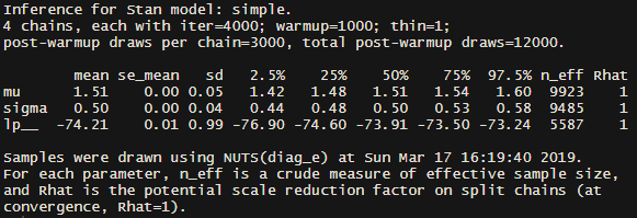
fit #Print a summary of the model to the console

#Exploration----
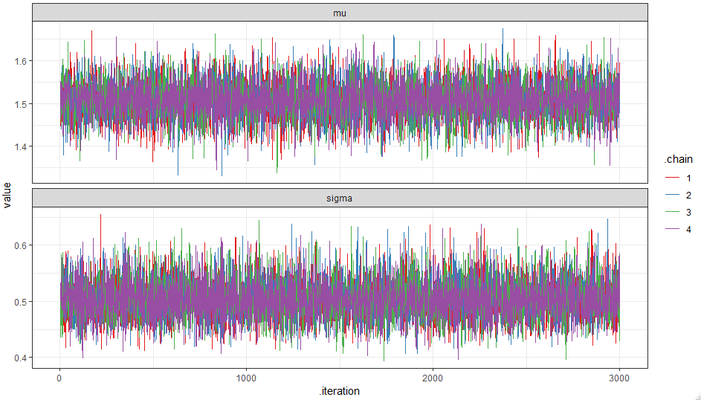
#The code below provides us a visual representation of the chains -- hopefully
# everything looks well mixed
fit %>%
tidy_draws() %>%
gather("parameter", "value", mu:sigma) %>%
select(.chain, .iteration, parameter, value) %>%
mutate(.chain = as.character(.chain)) %>%
ggplot(aes(.iteration, value, color = .chain)) +
geom_line() +
facet_wrap(~parameter, nrow = 2, scales = "free_y") +
scale_color_brewer(palette = "Set1") +
theme_bw()

Hopefully your fit object prints something like this (not exactly alike, just pretty close):

And your ggplot2 figure looks something like:

Setup for running a model on Teton

A note on paths

When using R interactively on Teton, wherever you launched R will be treated as your working directory. I therefore always try to run scripts and paths from my home directory, for the sake of consistency, but also write references to file locations relative to my home directory in the script. In my case, my home directory is /home/jmercer4. If you ever want to get back to your home directory in Terminal use the command: cd ~. Think of this command as your ruby slippers, because it will always take you home, no matter where you are on a computing system.

My strategy for managing data/code on Teton is to have all my Stan & R code, and data to be fit, in a project-specific folder in my home directory. I then write all my outputs to a similar folder structure in my scratch folder. I do this in part because the scratch folder has a lot more space on it than my home folder, so I can generate some really big output files, which I can then summarize later using some helper functions. For the specific project I'm using for this tutorial, my folders look something like:

/home/jmercer4/projects/AStudentsGuide
- /code: This will have my .stan model and .R file that has the call to Stan.
- /data: This will contain the data I will be be importing to R, which will then be used to fit my model.
/gscratch/jmercer4/projects/AStudentsGuide: All outputs from my R file will be written here.

This is the reason for the path locations you see in the script below.

Writing an R script for use on Teton

This script is modified from simple.R for use with Teton. It will therefore be called: simple_teton.R. I've store my copy in the same folder as simple.R.

#Load library
library(rstan)

#Options----
setwd("~") #Makes sure paths are relative to my home directory
rstan_options(auto_write = TRUE)
options(mc.cores = parallel::detectCores())
cat("Cores available:", parallel::detectCores()) # Tells me how many cores were
# used during execution on Teton

#Load data----
data <- readRDS("projects/AStudentsGuide/data/simple.rds") # Reads in the data

#Run model----
#Compile the model.
simple <- stan_model("projects/AStudentsGuide/code/simple.stan")

#Fit the model.
fit <- sampling(simple,
chains = 4,
iter = 4000,
warmup = 1000, 
data = data)

#Check the model.
fit
# mu ~ 1.5
# sigma ~ 0.5

#Save----
saveRDS(fit, "../../gscratch/jmercer4/projects/AStudentsGuide/fit.rds")

Note: I'm using how ever many cores are available to me. We'll specify the number of cores to use in both the interactive and batch sessions, when we start really using Teton.

Copy data and code from your personal computer

Once you've prototyped a model that works on your personal computer, you want to copy that model, and any affiliated data, to Teton. We're going to do this scp (secure copy), but another useful command is rsync. Personally, I like having two terminal windows open for data transfer – one focused on my local machine and one focused on my remote account – because it allows me to instantly check if the data I've moved is actually where I think it should be. Alternatively, you can use Globus or other upload strategies (Teton: beginner's guide).

Move my entire folder to Teton:

Navigate to the local location of my code: cd /mnt/c/Workspace/Learning/LearningStan/AStudentsGuide
Use scp to recursively copy everything from my local folder to my remote folder: scp -r * jmercer4@teton.arcc.uwyo.edu:~/projects/AStudentsGuide/
1. You will be asked for a password and get a push notice when you transfer data.
2. A break down of the what the code actually means:
  1. scp: We are using the scp command
  2. -r: We want to recursively transfer files from our personal computer – not just the file/folder indicated next.
  3. *: I'm using a wildcard to say that I want to copy everything from my current (local) directory.
  4. jmercer4@teton.arcc.uwyo.edu:~/projects/AStudentsGuide/: This is where I want to send everything on Teton (remote).
Open another terminal window.
Login to Teton.
Navigate to the folder you sent your data to: cd projects/AStudentsGuide/.
We can recursively look through this folder to make sure that everything looks good using: ls -R: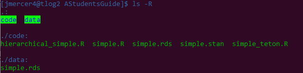
2. Yup. Everything looks good.
3. Note: /code/simple.rds is actually from the compiled stan program while /data/simple.rds is the contrived data we generated. Calling the data object that was a poor choice on my part.

Running your model on Teton

Interactively

In this section we're going to run our model interactively on Teton. This is probably fine for simple models that need a lot of memory, but that don't take much time or many cores. Since this is just a toy model, I'm going to log off the login node using most of the defaults:

srun --pty --account="ecoisolab" -t 0-02:00 --mem=10G /bin/bash

Note: You'll have to use your own account. Also, this will give you access to 16 cores, which is over kill for us, but shouldn't be an issue.

Now load all the required models to run both R and Stan. For R 3.5.2, this is done via:

ml swset/2018.05 gcc/7.3.0 r/3.5.2-py27 r-rstan/2.17.2-py27

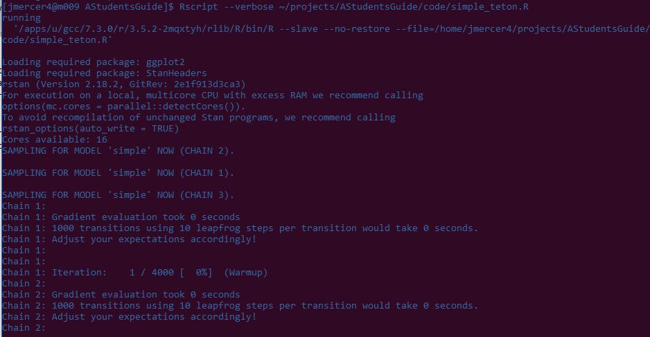
You should now be able to run your R script containing the code for calling Stan from R:

Rscript --verbose ~/projects/AStudentsGuide/code/simple_teton.R

A break down of this call:

Rscript: Using the Rscript command. You may see reference to a similar, but older command: R CMD BATCH. That version of calling a script is no longer recommended (it is used for lower level functionalities). For more on using the Rscript command: https://linux.die.net/man/1/rscript
--verbose: Prints a bunch of extra information to the console. I use this for troubleshooting.
~/projects/AStudentsGuide/code/simple_teton.R: The location/name of the script I want to run.

Output from your script should start to appear in your terminal window. Note that for this model, the part that will take the longest is compiling the model. The actual sampling runs in seconds. Also note that R/Stan is taking care of all the thread maintenance for us – we don't have to tell SLURM anything about how to manage our chains, they just run in parallel.

This is what the bottom of my script looks like:

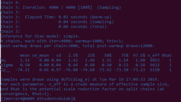
That output looks pretty dang similar to the model generated on my person computer!

Let's also make sure that it wrote the output somewhere so we can use it for other things:

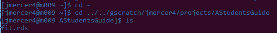
By the looks of it, a fit.rds file was indeed created, which we can now either manipulate further on Teton, or download to our personal computer.

Batch mode: Using Teton's job scheduler (SLURM)

This is the way you should use Teton when you think your jobs are going to take a while to run. This might seem a bit intimidating (at least it did to me), but it's not so bad when you've go the hang of it. Just a couple of slight modifications are needed to make our current R/Stan scripts run in batch mode. The main thing is writing a bash script that tells SLURM what to do, then telling the sbatch command to run our script.

Pathway 1: Small bash script with lots of arguments passed to `sbatch`

Writing and saving a bash script

Location of bash scripts

I like to centralize the location of my scripts, so they don't clutter my home directory. There are a bunch of different ways to do this, but for now I'm just going to make a folder in my home directory with an obvious name as to the purpose of the directory. That call is:

mkdir bash_scripts

Make a bash script

To make a bash script, I'll first make a file, again with an obvious name:

touch bash_scripts/simple_stan.sh

Note: Linux is an extensionless operating system, so the ".sh" doesn't actually do anything; the extension is just used to help us remember that the file is a bash script.

Now that the file has been made, we can edit it in a text editor, like Vim:

vi bash_scripts/simple_stan.sh

Add the following to the script and then save and exit:

#!/bin/bash

ml swset/2018.05 gcc/7.3.0 r/3.5.2-py27 r-rstan/2.17.2-py27
Rscript --verbose ~/projects/AStudentsGuide/code/simple_teton.R

Check that everything looks right by printing the text of the file to the terminal:

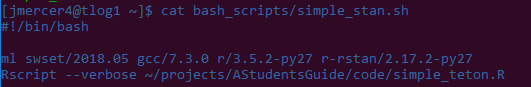
Everything looks good, so we can now run our job!

Pathway 2: A larger bash script with few arguments passed to `sbatch`

If you'd like to be a bit less verbose at the command line (because you know you'll use the same sbatch arguments each time your run your model), you can add some additional information to your shell script, which then gets passed to SLURM when you run the sbatch command. In this scenario your shell script will look like:

#!/bin/bash

#SBATCH --account=ecoisolab
#SBATCH --time=24:00:00
#SBATCH --nodes=1
#SBATCH --ntasks-per-node=4

ml swset/2018.05 gcc/7.3.0 r/3.5.2-py27 r-rstan/2.17.2-py27
Rscript --verbose ~/projects/AStudentsGuide/code/simple_teton.R

Then your sbatch call becomes:

sbatch ./shell_scripts/simple_stan.sh

Submit your job

Now that all the pieces and parts have been put together, we can run our job! I'm going to use the first "pathway" identified above, and therefore I will use the following command:

sbatch --account=ecoisolab --time=24:00:00 --nodes=1 --ntasks-per-node=4 ./bash_scripts/simple_stan.sh

When I run this command I get the following:

Notice that Teton lets us know that we have a job number/id, and what that number is. Once the job has been scheduled, Teton will produce a .out file, which contains our job number. Because I started my sbatch script from my home folder, Teton will place my .out file in the home folder.

Checking our job

The .out fill is simply what would have been printed to the console, had we run our R script in interactive mode – it is just a text tile. This is useful for seeing if our script ran successfully. Because the .out file is just text, we can check it at any point in time. However, if the job hasn't actually started then there won't be anything in the file. We can check the status of our job using the squeue command:

squeue -u jmercer4

In the above, I've simply told Teton that I want to see any jobs associated with my user account, but you could similarly see all jobs if you used no "flags" (i.e., got rid of the -u jmercer4 part of the call), or just focus on a single job using the -j flag (e.g., squeue -j 2500580), etc.

Once my file is finished running I want to check it and make sure it ran successfully. This can be done using the following:

cat ##jobid##.out

Where ##jobid## is the actual number of your job. In more concrete terms, you can see what happens when I cat one of my finished job files:

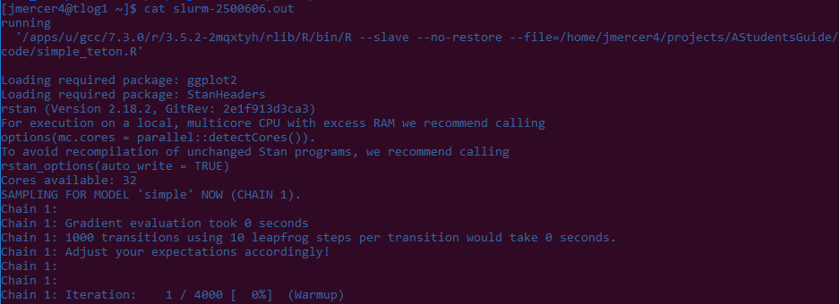
And that's it! You've just run a Stan model on Teton in batch mode!

UW Data Science Center

Working with Stan in R on Teton

Prerequisites

Suggestions

Other notes

What is Stan?

Model development

Strategy

Protyping a model on your local machine

A simple Stan model

Testing our model in R, using simulated data

Setup for running a model on Teton

A note on paths

Copy data and code from your personal computer

Running your model on Teton

Interactively

Batch mode: Using Teton's job scheduler (SLURM)

Pathway 1: Small bash script with lots of arguments passed to `sbatch`

Writing and saving a bash script

Location of bash scripts

Make a bash script

Pathway 2: A larger bash script with few arguments passed to `sbatch`

Submit your job

Checking our job

Related articles

Prerequisites

Suggestions

Other notes

What is Stan?

Model development

Strategy

Protyping a model on your local machine

A simple Stan model

Testing our model in R, using simulated data

Setup for running a model on Teton

A note on paths

Copy data and code from your personal computer

Running your model on Teton

Interactively

Batch mode: Using Teton's job scheduler (SLURM)

Pathway 1: Small bash script with lots of arguments passed to sbatch

Writing and saving a bash script

Location of bash scripts

Make a bash script

Pathway 2: A larger bash script with few arguments passed to sbatch

Submit your job

Checking our job

Related articles

Pathway 1: Small bash script with lots of arguments passed to `sbatch`

Pathway 2: A larger bash script with few arguments passed to `sbatch`